In dynamic resource allocations and load balancing, one of the most well-known and fascinating algorithms is the so-called “power of two random choices,” which proposes a very simple change to the random allocations that yields exponential improvement. I was lucky enough to have implemented this very technique on a gigantic scale to improve the resource utilization of AWS Lambda, and yet I struggled to “feel” it intuitively for a long time.

In this article, I’d like to share my mental model for understanding this algorithm which also helps build a good intuition for many other advanced techniques in this area.

Update: I have a follow-up article that shows applying this algorithm in a more complex model than ‘balls in bins’.

What is Load Balancing?

Let’s say you run a large-scale AI bot service like ChatGPT. You have thousands of servers with expensive GPUs generating text based on user prompts. Now if your algorithm was routing about 80% of incoming requests to only 20% of servers, that 20% of servers would be quite busy, and the requests hitting those servers will likely have to wait for quite some time to see a GPU. On the other hand, 80% of cold servers are poorly utilized and waste many precious GPU hours. This is what we call bad load balancing.

On the other hand, if all your servers are roughly taking equal load, you are answering your requests in near-optimal time and not overpaying for resources. Moreover, you can easily “right size” your fleet — expand it to improve response time or contract it to reduce cost.

Power of Two Random Choices

There’s a simplified model to think about load balancing. You have an infinite stream of balls (representing requests) and N bins (representing servers). Your job is to assign each incoming ball to a bin such that you keep the allocations across all bins as equal as possible. A real-world problem is much more complex than this, but this simplification will do for now.

One of the easiest strategies for balls-in-bins is to pick a bin and place the ball in it randomly. If we use uniform random picks, all outcomes are equally likely for every pick, so we’d expect all bins to be roughly equally filled.

The other approach — you pick two random bins instead of one and place the ball in the emptier one. This is the so-called “power of two random choices” approach — we’ll call it “best of two” for short.

Let’s run a simulation placing one million balls into 1,000 bins with both of these approaches — the best case for the end state being 1,000 balls in every bin. As per the histograms of bins below, the difference is quite dramatic.

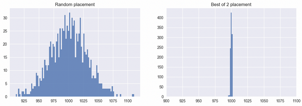
The random placement results in a wide distribution ranging roughly from bins with 900 balls to 1,200 balls, while the best of two placements yield a much tighter distribution between 995 and 1,002.

What’s Wrong with Just Random?

You likely recall hearing about the “Central Limit Theorem” in some math class. It’s fundamental to statistics and roughly states that the sums of independent samples from any random distribution (like our uniform distribution) are normally distributed.

Let’s try to “feel” it more intuitively, though. You have ten bins — all empty initially. You take the first ball and roll a ten-faced dice and get “1.” So bin #1 now has one ball while all others are still empty. You have to now place a second ball. You roll the dice again. Since this dice roll is completely independent of the first roll and has no “memory” in any way, all outcomes are still equally likely even though the bins are now imbalanced.

Now for bin #1 to not become a further problem for us by getting a second ball while several other bins are empty, we are not allowed to roll “1” on our dice for the next nine attempts. The probability of that is (9/10)⁹, which is just 39%, so it’s more likely than not that we will roll a one before that and make things more imbalanced.

That said, since we randomly place 100 balls into ten bins, we’d still expect the per bin count to be ten, but since this is a probabilistic system, the expectation means the average of the distribution. Therefore, we’d see most bins close to ten, some significantly underfilled, and some significantly overfilled, resulting in a symmetric normal distribution, as seen in Figure 1.

Another way to look at this: each bin’s placement history can be represented as a list of X’s with Xth ball being placed in that bin from the stream. The difference between the consecutive X in this list can be less than ten or greater than ten or exactly ten. As a result, the length of the list can be less than ten, greater than ten, or exactly ten.

However, since we only placed 100 balls, for all the “less than ten-ness” in the world, there has to be an equal “greater than ten-ness” resulting in the average behavior of ten with a symmetric distribution around it. This pattern of arrivals also has a well-known distribution called geometric distribution.

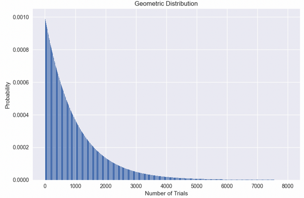
The plot in Figure 2 shows the shape of a geometric distribution for our previous example of one million balls in 1,000 bins. The geometric distribution is a long-tailed distribution which means it packs more probability between [0, mean] but sees much larger than mean values down the line, albeit with lower probability. The mean, in this case, is 1,000, but we see as many as 8,000 attempts before seeing the same bin twice!

Good vs. Bad Placements

Before we jump into optimization, let’s try to define an objective function for good placements. In practice, doing this is incredibly complex, but for our toy example, it’s relatively easy. We start with N bins and want to place M balls onto these. We define the number of balls on the nth bin as Sn. Globally. We define Smin and Smax as the number of balls in the emptiest and fullest bin, respectively.

Initially, the Sn for all bins is 0. Therefore Smin and Smax are 0 as well. As soon as we place a single ball in any bin, say bin #1, S1 is 1, Smin is 0, and Smax is 1. Now if we have optimal placement, our Smax should never be more than Smin + 1.

For example, if n = 10, S1 = 1, and S2 to S10 are 0, there’s no reason whatsoever to make S1 = 2 before placing it in nine empty bins first. Only when the Smin = 1 (which will happen when all bins have one ball) would an optimal algorithm would take the Smax to 2. Therefore, Smax — Smin > 1 is a sign of bad placement. We can visualize this as concentric circles or orbits. Smin is your center and Smax increments by one per orbit. The farther your orbit, the worse your placement.

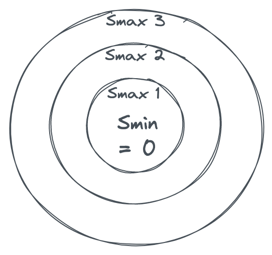
In other words, any algorithm that makes it really, really hard for Smax to get several orbits away from Smin is a good placement algorithm.

Best of Two Placement Analysis

My mental model for the best of two placements is that it creates a horrendously complex maze between the orbits in Figure 3 that gets increasingly complex as we try to get to higher orbits. As a result, the placements have a hard time reaching those undesired states.

Let’s go back to our former example of ten empty bins. The first ball is placed in bin “1,” so we are in orbit 1. With random placements, there’s a 10% chance of getting into orbit 2 (i.e., pick bin “1” again). When you are in orbit 2, there’s still a 10% chance to go to orbit 3. Basically, there’s always a 1/n probability we’ll make our placements worse by 1 in random placement.

Now let’s analyze the best of two. Let’s say bin 1 and bin 2 contain one ball each. Now, the probability that we will upgrade to orbit 2 is:

1. We have to pick one of the two filled bins on the first draw, which is 2/10.
2. We have to pick the second one on the second draw, which is 1/9.

When these conditions are met, we will be forced into orbit 2. Combining the probabilities, we get a probability of 1/45 or roughly 0.02 vs the 0.1 from random placement. That’s good, but I am not impressed yet, so let’s think about getting to orbit 3.

For random placement, you have to hit bin “1” to get to orbit 2 and once more to get to orbit 3, so the probability of the shortest path to orbit 3 is 0.01.

Again, with the best of two algorithms, let’s start with “1” and “2” bins containing one ball each. The following events depict the fastest path to orbit 3:

1. Pick one of the filled bins: 2/10
2. Pick the second one: 1/9 — we are in orbit 2 as we place the ball in one of these two, same as before.
3. In the next draw, we draw the orbit 2 bin: 1/10
4. Then we draw the lonely orbit 1 bin: 1/9 — This now puts both bins in orbit 2.
5. Now we again draw both of these bins: 2/10 * 1/9 — This will finally take one of them to orbit 3.

If we multiply all these probabilities, we get 0.0000054 vs 0.01. We’re now seeing the maze I was talking about earlier. Note that this is the probability of the shortest path, and there could be other paths that are longer but can be hit with a higher probability, but you get the idea.

I’d love to go on and show the probabilities for orbit 4, 5, etc., but I lack the math skills. I am, after all, a mere programmer. If you are like me and your programming skills are way better than your math skills, you really want to make friends with the Monte Carlo simulations. In simple terms, a Monte Carlo simulation is where, instead of solving a problem mathematically, you run many, many instances of that problem on a computer with random input.

Thanks to the law of large numbers, if your sample size is large enough, your results will be pretty close to the mathematical results — close enough to prove your point.

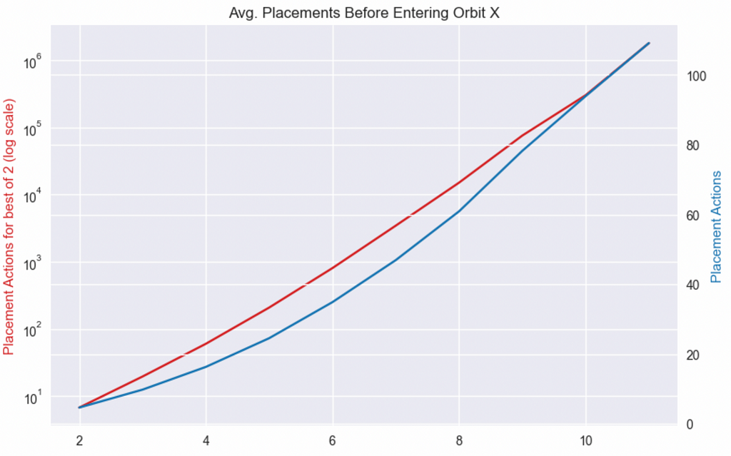
In this case, instead of dealing with probabilities, we run 10,000 experiments of seeing how many placements it takes on average before we get to orbit 2, 3…11 with either algorithm.

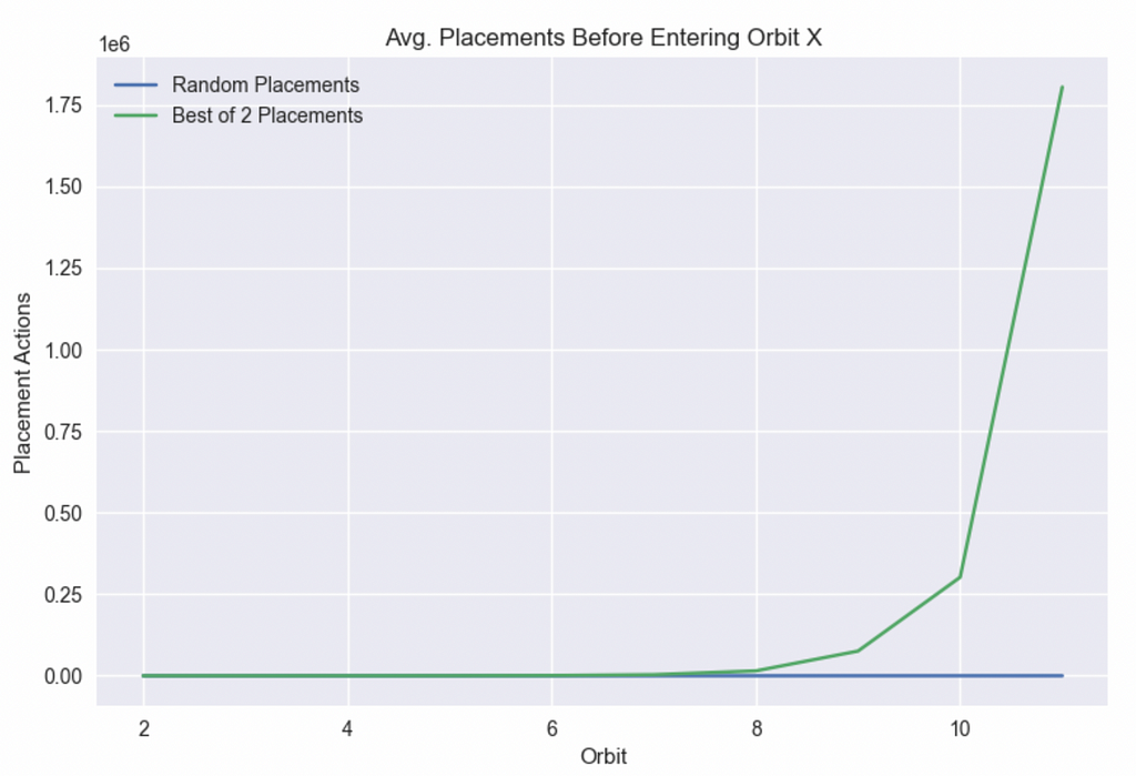
Anybody familiar with exponential growth will recognize the shape of the chart above. Once you get past the first couple of orbits, it gets incredibly hard to get to higher orbits with the best of two since the difficulty grows exponentially. In contrast, the difficulty of random placements increases linearly.

To compare the growth patterns, let’s plot the best of two on a log scale and keep random placements on a linear scale.

Conclusion

In this article, we saw how the best of two random choices algorithm exponentially improved the quality of placements by making it probabilistically very, very hard to make bad placements beyond a certain point.

On our way there, we also built an intuition for the Central Limit Theorem as it relates to this problem and learned how Monte Carlo simulations can help us get solutions to pretty hard math problems with a bit of programming and lots of patience.

This article was meant to help build intuition for some basic concepts in resource allocation — a topic I deeply love. As I have implemented this and a lot more advanced techniques at scale, I’d love to dive into a lot more topics in future articles. I may write about ways to generalize this algorithm when there are multidimensional balls with different CPU/memory needs. Even if the bins aren’t all alike, bins are often replaced. How can we generalize the best of two to the best of k, find a good k, etc?

Load Balancing: The Intuition Behind the Power of Two Random Choices was originally published in The Intuition Project on Medium, where people are continuing the conversation by highlighting and responding to this story.