In my previous writing on load balancing, we applied various techniques to the simple “balls in bins” model. Simple models are great because they are easier to understand and easier to manually debug if needed. However, if your interest in the subject is beyond just academic, you want to graduate to higher-fidelity models to make better contact with reality.

For this post, I want to expand the “balls in bins” model into one where we consider two (usually) most important dimensions of workloads: CPU and memory utilization and demonstrate how that introduces many new problems you didn’t have to solve in the previous model. We will see how we can adjust our favorite algorithms from before to work with this additional complexity.

So like before, we have N worker machines. They all have C total CPU seconds to spend every second and M gigabytes of RAM. A workload needs c seconds of CPU every second and m gigabytes of RAM to run. Since the workload needs to run on a single worker, obviously m ≤ M and c ≤ C. Once placed on a worker, we assume that the workload acquires all needed resources at once and keeps using them till the end of time. I’m sure you realize these details aren’t very realistic either but we can’t just pile up all complexity at once.

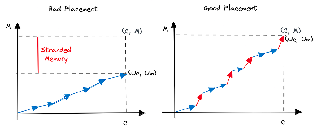
One way to visualize this problem is using vectors. Imagine every workload as a vector of [c, m] and the worker itself as a large vector of [C, M]. The sum of all workloads currently running on the worker constitute the utilization vector. Let’s call it [Uc, Um]. Once again, Uc ≤ C and Um ≤ M.

If you fill too many CPU-hungry workloads on a worker, you risk exhausting the CPU while a lot of memory is unclaimed and vice versa. These resources are often called stranded resources. You want to globally minimize the stranded resources because in a sense these are the resources you are paying for but not getting paid for. In other words, if you have a lot of stranding, you need a much larger fleet than the sum of all Cs and Ms to handle your global aggregate workload, which is sum of all cs and ms.

Simulation

The simulation in this case is a little more nuanced because we have to generate the workload data now. In reality, this is your actual traffic. If you have very homogenous workloads, your load balancing problem is quite easy as it resembles “balls in bins” model as we didn’t think of balls with different shapes and sizes there. You just have to choose the worker size carefully (e.g. between EC2 M, C and R instances) and you are good to go. However, not everyone is this lucky. Especially when you are running 3P code, as I was back in my Lambda days, you have to deal with a huge mix of very different shapes — some of them pathologically bad. This produces many very interesting placement problems: some of which we’ll discuss in this post and some we will leave for later.

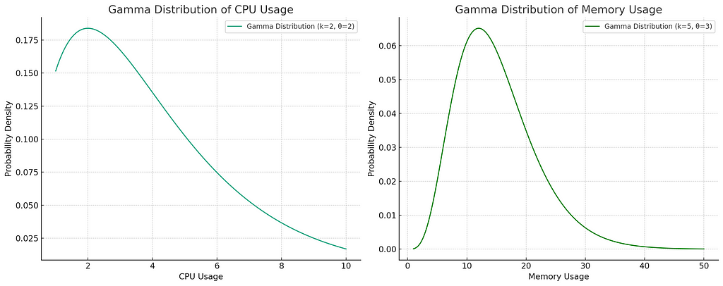
In a real world setting, you’ll fit a distribution to your real data and then work with that distribution in simulations. In absence of that, we will make up some distributions out of thin air (with all that CPU heat you know). The CPU and memory distributions I am most familiar with are where a large bulk of workloads fall in low utilization bucket while a smaller number end up using dramatically more resources in one of the dimensions — these are the above mentioned pathological workloads. Gamma distribution is great to model such workloads — in fact it can model many things and is often my go-to distribution. We’ll use following distributions for CPU and memory.

With this, we are ready to place 100k workloads on 10k workers assuming 50 CPU cores (so supports 50 seconds of CPU time every second) and 250GB memory. Initially, we will use random placement — pick any worker randomly and try to place on it. If there’s no space, we mark it as a failed placement.

We saw about 6000 failed attempts with a very large number of workers nearly full in CPU which means most workers had a lot of stranded memory. Sadly, there were also some workers with stranded CPU.

Power of two random choices

For those who have read my previous articles, the result should be no surprise. Random placement isn’t great for resource distribution. However, “power of two random choices” is supposed to be the magical algorithm that fixes everything. So let’s apply it here just like before — we will look at two random workers and choose one with fewer workloads.

Well that’s a lot better! None of the workers are full in memory so we did not strand any CPU. We did still strand a lot of memory though as 500 or so workers have all the CPU consumed but it’s down from 1100 so still a lot better. Failed placement count is smaller by 50%.

Other objective functions

So power of two random choices does work but it’s not as powerful as before with “balls into bins”. Let’s see if we can fix that with a different objective function than “number of workloads”. The rationale is since the workloads are far from uniform, the number of workloads does not tell the whole story. Our objective isn’t making sure all workers have equal number of workloads (in that job, we did spectacularly well based on the third graph in figure 4). Instead, we want to make sure they are all “filled” uniformly in both resources.

L2 norm

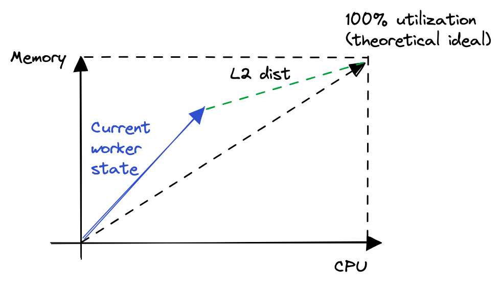
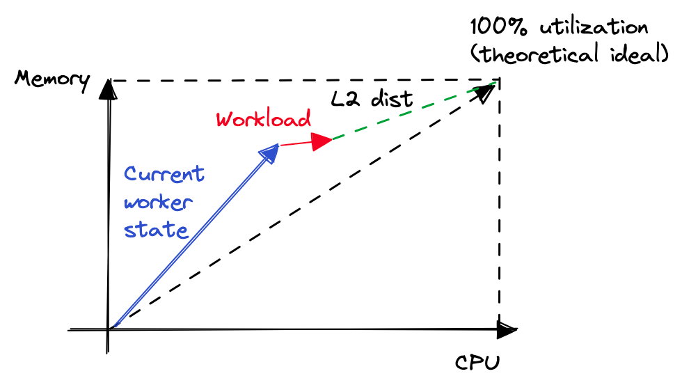
In linear algebra, we have the idea of norms to compare how far two vectors are from each other. The second norm, or L2 norm, is same as the Euclidean distance and is a very popular metric for geographical and geometrical problems. Since we already know that the ideal placement will occur when (Uc, Um) == (C, M), we can say that closer the (Uc, Um) is to the (C, M), better is a worker placed. There are a few caveats when new workers are introduced in an already full fleet but we’ll leave that aside for now. So with that knowledge, we will now change our objective function to placing in a worker with larger distance of utilization from ideal — hoping that adding this workload there will make things better. Note that when calculating utilization, we definitely want to do it as a percent or other normalized form and not absolute values.

That’s much better. While our workloads per worker distribution is wider, our CPU and memory distributions are looking a lot better reducing the stranded resources and failed placements.

Can more data help?

Assuming we have a way of knowing how much resource the given workload is going to need — maybe because the customer has to specify in advance or maybe because you have a data pipeline to remember older values. In that case, instead of just calculating the emptiness of the worker, we can calculate emptiness when the workload is placed.

That’s a lot better! Our failed placement count went down to 1100 from 1400 and number of full CPU workers went down from ~350 to ~220.

As before, we have all the levers at our disposal for tuning the algorithm. For example, here’s what happens when we use k=5 instead of k=2.

We’re almost done now but maybe there’s something even better.

Leaning more on your data

By now, it must be clear that we’re having a lot harder time not stranding memory than not stranding CPU. This means CPU is the harder dimension to balance for us. In that case, why not put all the focus on CPU and just ignore memory? So basically we’ll do a best of 5 random choices with objective being to choose the worker with least amount of memory left.

So close! We pretty much solved our memory stranding problem here but also started stranding a little bit of CPU in the process. Failed placements went further down so by-and-large we’d consider this a better outcome.

Again, note that this type of radical objective function won’t always work which is why it’s important to understand your data well and simulate before putting things in production.

Conclusion

In this post, we expanded our model a little and dealt with some realistic problems with multi-dimensional placements. We also modified our favorite “power of two random choices” algorithm with better objective functions. In terms of a good model for testing real algorithms, we are just scratching the surface though. In next posts, we will un-simplify various aspects from this model and update our strategies to meet the new requirements.

Load Balancing: A More Realistic Model was originally published in The Intuition Project on Medium, where people are continuing the conversation by highlighting and responding to this story.