In my previous post, we built an intuition for how the “Best of two” algorithm improves load balancing by making it extremely hard to get too far from the optimal placement. In this post, we will look at a counterintuitive optimization that’s easy to implement and guaranteed to make your placements a lot more efficient. As always, we will build a solid intuition for why it works which will help think about similar problems in the future.

The algorithm discussed in this post comes from this paper from professor Vöcking. I highly recommend the paper for a more rigorous mathematical analysis.

What’s the Optimization?

As a recap, the algorithm we saw in the previous post is: sample two bins randomly without replacement (meaning don’t select the same one twice) from your fleet of bins and place the ball in the emptier one. If they are equally full, then pick any one of them randomly. We can easily generalize this algorithm from “best of two” to “best of K” random choices where K ≤ N but typically a small number like 2, 3 or 5.

Let’s change this approach slightly. Instead of picking your K samples randomly from the entire fleet, create K logical partitions in your fleet e.g. at K=2 and N=100, you’d put bins 1–50 in first partition and 51–100 in the second. Now, take a random sample from each partition — rand[1, 50] and rand[51, 100]. Now, compare the sampled bins. If one bin is emptier than all other bins, choose it just like before. However, if there’s a tie for the lest loaded bin, always place in the one from the left-most partition.

Previously, we used the concept of “orbits” to determine effectiveness of a load balancing algorithm. If you are in the Nth orbit, you are N away from the ideal placement in terms of max(bin_load)-min(bin_load). An algorithm is better if it requires more steps on average to get into the Nth orbit. Let’s compare the base and optimized algorithms for orbit [3..5] and K values [2..5]. The fleet size is 10,000.

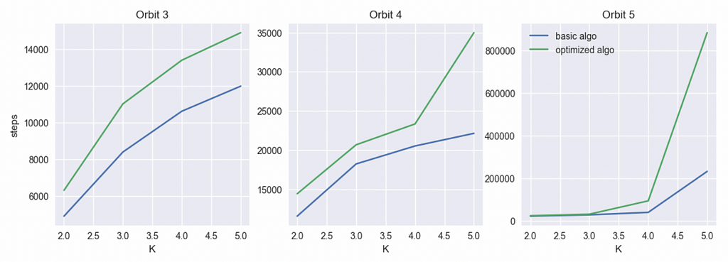
Turns out the optimized algorithm performs substantially better at all orbits and especially better at high orbits when K is high. In other words, the optimization always makes it harder to do suboptimal placements but if the sample size is sufficiently large, making majorly bad placements becomes so improbable, it approaches impossibility.

The paper calls this “Always Go Left”. We’ll refer to it as AGL in this post.

Let’s Talk About K > 2

Before dealing with the elephant in the room for why a worse-sounding algorithm actually works better, let’s first deal with another issue of how a larger K relates to the efficiency of our algorithms. Intuitively, it makes sense that if you make your decision based on a larger sample, you’ll make better decisions. In fact, if your K=N, you are guaranteed to make optimal decisions. In our orbit model, we can say that with 100 bins, at K=100, you’ll need infinite moves to get to the orbit 2. Let’s look at how this efficiency scales though from K=2 to K=99.

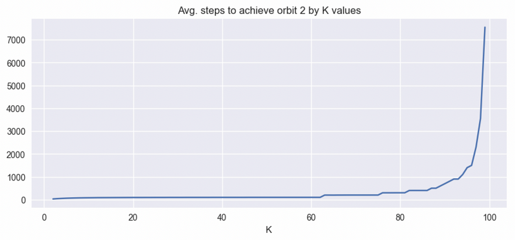
Turns out, most of the benefits from a large K are concentrated towards the higher side of K. We see this pattern across the board for higher orbits as well where there’s a value of K beyond which entering that orbit is highly improbable but the gains towards that stage scale sub-linearly.

In practice, using a large K can be difficult because of the additional overhead of having to reach out to a large number of servers. In high-churn environments (typically the type of environments where you’d want this type of algorithms) and with many independent placement servers, taking too many samples reduces the fidelity of your sample as what you see as the “best candidate” is likely also seen by many other servers as the best candidate and it’s bombarded into a very different state by the time the workload materializes. Speaking from experience, this is especially pronounced when you bring new servers into your fleet. If your placement servers sample too much, they’ll all find this new server fully empty and fill it indiscriminately to the point it’s be really poorly placed. This continues over time and makes your placements look bad.

That said, for a large fleet of 10k or so servers where tasks aren’t typically stuck for a long time, a moderately large K such as 3, 5 or 7 is doable and actually quite beneficial. An A/B test is a great way to find the right value.

How does the AGL optimization change K > 2

Next, let’s examine what the AGL optimization looks like on the plot in the figure 2.

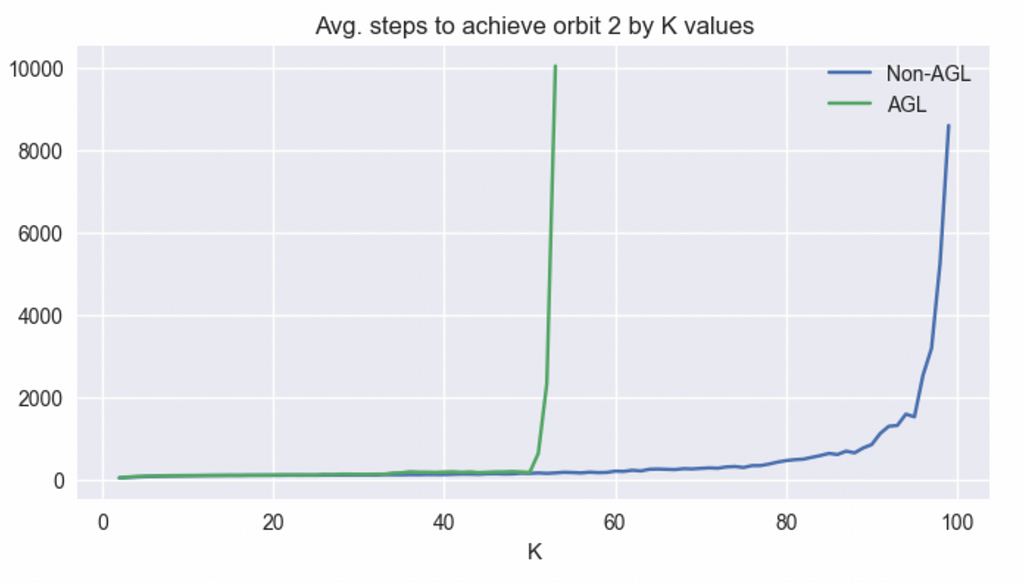
Turns out, AGL looks fairly similar to the base algorithm for smaller Ks but diverges and approaches the apparent probabilistic wall much more quickly.

The paper that proposes this algorithm shows that the worst placed bin in a regular best of K is filled up to O(ln.ln(n) / ln(k)). With AGL, this changes to O(ln.ln(n) / k). Notice that the denominator term changes from ln(k) to just k which is of course an exponential increase. As k gets larger, the difference between ln(k) vs k grows dramatically which is why the placements look much better at large k when you use AGL as seen in figure 1 and 3.

Intuition for AGL

First, let’s debunk a common misconception a lot of people including me implicitly hold. AGL indeed makes the left-most partition fill up with priority so at any given time, you’d expect your left partition more full. This sounds to some like bad placement — which isn’t necessarily true. For example, [2, 2, 1, 1] is a much better placement than [3, 0, 0, 3] even though the latter is symmetric and former isn’t. Our goal is to make sure we don’t end up in the high orbits. Creating some sort of symmetry among our servers is not in any way important.

The paper uses a technique called witness trees to prove an upper bound for AGL which is a very similar to my concept of orbits although orbits are more of a tool for building intuition while witness trees actually help prove things. For building a good intuition however, I’d like to jump into the mechanics of this algorithm by analyzing a very simple case deeply: placing 100 balls in 100 empty bins.

Let’s start with the simple case of K=2. It should be somewhat obvious that a few initial samples will be (0, 0) and we will start filling the left partition. At one point, there will be enough “1”s on the left side and the balance of probability will shift more towards (1, 0) samples and we will start filling the right partition more aggressively. When enough bins on the right have been filled, the left side will be preferred again and so on and so forth. Below is the plot of a single run of placing 100 balls in 100 cold bins:

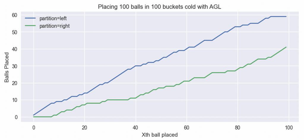
The plot below is similar to figure 4 but instead of a single run, I averaged runs of 100 such placements so we get cleaner patterns:

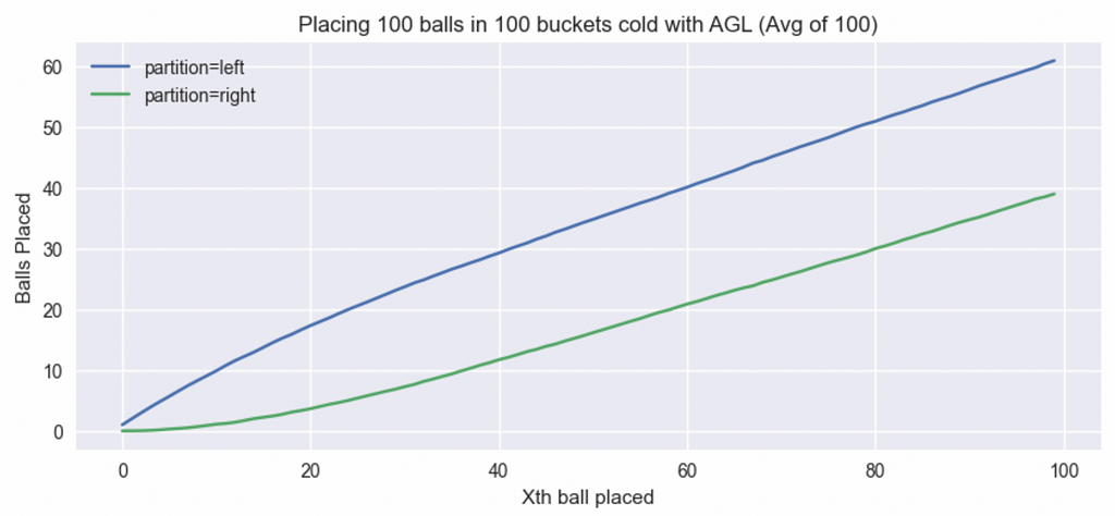
All said and done, we get ~60 balls in left partition and ~40 in the right partition. Again, balancing partitions isn’t our goal so this is fine. On the plus side, it’s extremely difficult to have a bucket with 3 balls.

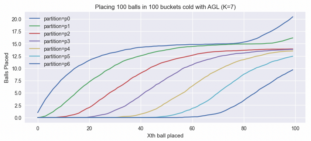
Let’s now look at another example of K=7. With so many partitions, we get a better idea of the generalized working of this algorithm. Again, the partition 1 starts filling first followed by partition 2 followed by 3, 4, …7. As soon as 7 fills to a critical point, 1 starts filling again and so on. See figure 6 for a 100 attempt average of filling 100 buckets with 100 balls each time with K=7.

Comparison with round-robin

Now that we understand how the partitions fill in AGL, one can’t help but relate this to the round-robin algorithm at partition level. While the partitions don’t quite fill one at a time, there’s a sense of order as the partitions enter a higher orbit one after the other. It’s literally impossible for any bin in a higher partition to enter an orbit before at least one bin in all partitions before have. In our K=7 example above, this means that about 85% bins are safe from prematurely entering a higher orbit. This also explains why a larger K makes this algorithm so much more effective.

In case you are wondering why we don’t just implement a round robin approach here, remember that in a real world setting, we will have maybe tens of placement servers placing against tens of thousands of worker servers that are constantly getting rotated and new workers coming in. With so much going on, an algorithm that doesn’t look at the worker state doesn’t end up doing well over time. AGL, while it has some nice properties from round-robin, doesn’t suffer from these problems and can be nicely implemented independently from multiple placement servers.

Caution on partitioning

While AGL improves the overall placement state of your fleet, the servers in your left partition will be slightly more loaded than the rest of the partitions. This is not a problem as long as you assign servers to your partitions randomly. If you create your partitions by which AZ the server belongs to for example, that can be a problem as it might make losing that AZ worse. Remember that a partition in AGL is not a shard or a unit of availability but just a simple algorithmic trick. Even if you do have shards, avoid using those as your AGL partitions.

For every incoming worker, you can check the emptiest partition and tag it in a database so it stays consistent.

Conclusion

Building on the previous post on the power of two random choices, we learned about two important concepts: the always-go-left optimization and the sample size K > 2. We also saw how ALG maximizes the efficiency gains from choosing a large K. We built a good intuition for why AGL works and learned a few practical tips for implementing AGL in your fleet to realize the gains.

In the subsequent posts on this topic, we will get out of our over-simplified balls-in-bins world and learn tricks for building a real life load balancing system at scale.

Load Balancing: A Counterintuitive Improvement to the Best-of-K Algorithm was originally published in The Intuition Project on Medium, where people are continuing the conversation by highlighting and responding to this story.